Statistical Inference with R
Linear & Logistic Regression Modeling
Building and interpreting regression models for continuous and binary outcomes
Dan Kerchner · George Washington University Libraries & Academic Innovation · Fall 2026
Upcoming R Workshops (Fall 2026) 🗓️
- Oct. 1 (Thurs.), 1pm-3:30pm | Farther into R: More R for Data Analysis
There will be more in the Spring!
📅 Find all GW Libraries workshops and events at library.gwu.edu/events
What are we actually doing?
Linear Regression Model
\[ Y = \beta_0 + \beta_1X_1+\beta_2X_2 + ... + \beta_nX_n \] where \(Y\) is a continuous variable.
(and an interaction term might look like \(\beta_{1,2}X_1X_2\))
Interpretation
\(\beta_0\) = Mean \(Y\) when \(X_i\) values are \(0\)
\(\beta_1\) = Mean change in \(Y\) for a 1-point increase in \(X_1\), adjusting for other \(X_i\) variables
Correlation between dependent & independent variables
Pearson correlation (\(\rho\)) measures strength and direction (+/-) of linear association between \(X_i\) and \(Y\). Ranges from -1 to +1.
If the relationship looks non-linear (but monotonic) then Spearman correlation should be considered.
\[ H_0: \rho = 0 \] \[ H_1: \rho \neq 0 \]
Valid if joint distribution of X, Y is bivariate normal.
Linear Regression Assumptions
- Observations are independent
- Linearity
- Homoscedasticity
- Normality
GLMs – Generalized Linear Models
\(g(\mu) = \beta_0 + \beta_1X_1 + \beta_2X_2 + ... + \beta_nX_n\)
where \(\mu = E(Y)\)
Common link functions
\(g(\mu) = \mu\)
\(g(\mu) = log(\mu)\)
\(g(\mu| = log(\frac{\mu}{1-\mu}) = logit(\mu)\)
(Binary) Logistic Regression Model
\(log({\frac{p}{1-p}}) = \beta_0 + \beta_1X_1 + \beta_2X_2 + ... + \beta_nX_n\)
where
\(p\) = Probability of \(Y = 1\)
\(1-p\) = Probability of \(Y = 0\)
Interpretation
\(\beta_i\) = log OR (odds ratio) for having \(Y=1\) for a 1-point increase in \(X_i\), adjusting for other predictors
\(e^{\beta_i}\) = OR (odds ratio) for having \(Y=1\) for a 1-point increase in \(X_i\), adjusting for other predictors
Binary Logistic Regression Assumptions
- Binary outcome (0, 1)
- Each predictor is linearly related to the log odds of the outcome
Inference for regression modeling
Confidence Interval
95% CI for \(\beta\) = (0.44, 0.49)
Hypothesis Testing
\(H_0: \beta = \beta_0\) <- Null Hypothesis
\(H_A: \beta \neq \beta_0\) <- Alternative Hypothesis
p-value: Chance that we’re rejecting \(H_0\) when we shouldn’t be
Today’s Goals
Learn to use R to read in data and conduct regresison analysis with associated inference tests
- Checking assumptions
- Visualizing the data
- Computing p-values, regression coefficients, confidence intervals, and (for logistic models) odds ratios
2 Scenarios
- Linear Regression (continuous outcome)
- Logistic Regression (binary categorical outcome)
(with both continuous and categorical predictors)
Data Set #1: Siddarth et al., 2018
Siddarth P, Burggren AC, Eyre HA, Small GW, Merrill DA (2018) Sedentary behavior associated with reduced medial temporal lobe thickness in middle-aged and older adults. PLoS ONE 13(4): e0195549. doi.org/10.1371/journal.pone.0195549
- Examined associations between sedentary behavior and medial temporal lobe (MTL) subregion integrity
- 35 non-demented middle-aged and older adults
- Measured physical activity levels w/questionnaire
- Measured MTL thickness w/MRI scan
- Adjusted for age

Data Set #2: Framingham Heart Study
- framinghamheartstudy.org
- Long-term prospective study of the etiology of cardiovascular disease among a population of subjects in Framingham, MA
- Began in 1948 with 5,209 subjects
- Is the source of the term “risk factor”
- Over 3,000 peer-reviewed papers published based on this study
- Participants were each followed for a total of 24 years for cardiovascular events (heart attack, stroke, death, etc.)
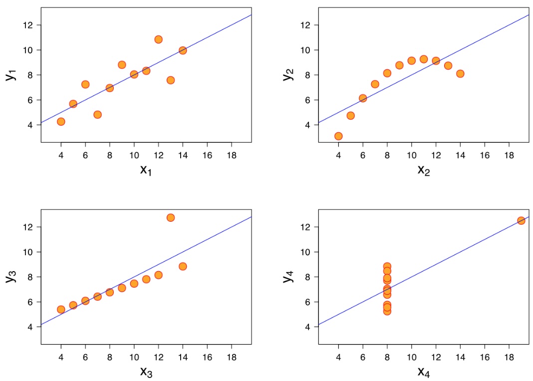
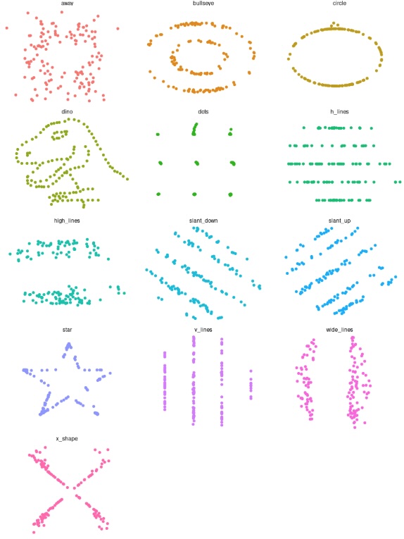
First, visualize the data! Is a linear model even the right one?
Anscombe’s Quartet
Datasaurus Dozen
Some R packages and functions for regression
lme4- Linear mixed-effects models
MASS- Model selection
ts(),arima()- Time series object, model (part ofstats)
forecast- Forecasting for time series and linear models
mice- imputation of missing data
medflex- mediation analysis
splines2- regression spline basis functions
survival- survival analysis; JM - joint modeling
Thanks! 🎶 🙏
Dan Kerchner | George Washington University Libraries
kerchner@gwu.edu
Stats & Coding help @ GW:
| me | R, Python, etc. | calendly.com/kerchner |
| Academic Commons Data Consultants | R, Statistics, Python, SAS, Excel, etc. | go.gwu.edu/DataConsulting |
| LAI Software developers | Python, web apps, HTML, etc. | calendly.com/gwul-coding |
These slides: kerchner.github.io/r4stats/regression
Code: github.com/kerchner/r4stats in the regression/R folder
R LibGuide: libguides.gwu.edu/r_stats
Statistical Inference with R · GW Libraries & Academic Innovation · kerchner.github.io/r4stats