library(forcats)
library(dplyr)
Attaching package: 'dplyr'The following objects are masked from 'package:stats':
filter, lagThe following objects are masked from 'package:base':
intersect, setdiff, setequal, unionA data variable can either be continuous or categorical. Continuous variables can take on any value within a range, while categorical variables can only take on a limited number of values.
Let’s look for a moment at different types and subtypes of variables that we might have:
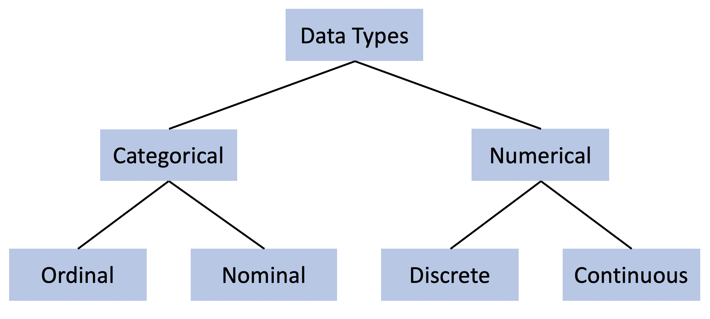
Let’s focus for a moment on Categorical data. Categorical data might have values that are either text or numeric:
'control', 'treatment''red', 'blue', 'green''good', 'better', 'best'0, 1 (e.g. for control and treatment)1, 4, 2 (e.g. for red, blue, green)1, 2, 3 (e.g. for good, better, best)In R, categorical variables are called factors. Factors can be either ordered or unordered. So 'control', 'treatment' would be an unordered factor, while 'good', 'better', 'best' would be an ordered factor.
forcats library 
The forcats library, which is part of tidyverse, provides a number of elegant and useful functions for working with factors. Let’s load it now. We’ll also need dplyr for data manipulation.
library(forcats)
library(dplyr)
Attaching package: 'dplyr'The following objects are masked from 'package:stats':
filter, lagThe following objects are masked from 'package:base':
intersect, setdiff, setequal, unionLet’s say we have a data frame that contains some categorical data, like this:
corporations <- read.csv('data/corporations.csv')
str(corporations)
'data.frame': 31 obs. of 10 variables:
$ Company.Name : chr "Apple Inc." "Microsoft Corp." "Walmart Inc." "JPMorgan Chase" ...
$ Industry : chr "Technology" "Technology" "Retail" "Finance" ...
$ Corporation.Type : chr "C Corporation" "C Corporation" "C Corporation" "C Corporation" ...
$ Tax.Treatment : chr "Corporate tax" "Corporate tax" "Corporate tax" "Corporate tax" ...
$ Ownership.Limits : chr "Unlimited shareholders" "Unlimited shareholders" "Unlimited shareholders" "Unlimited shareholders" ...
$ Governance.Structure : chr "Board of Directors" "Board of Directors" "Board of Directors" "Board of Directors" ...
$ Public.or.Private : chr "Public" "Public" "Public" "Public" ...
$ NAICS.Code : int 334111 511210 452311 522110 312111 519130 454110 336111 541330 445110 ...
$ X2024.Estimated.Revenue..USD.: num 3.91e+11 2.45e+11 6.48e+11 1.78e+11 4.71e+10 ...
$ Number.of.Board.Members : int 8 14 12 12 14 11 11 10 10 9 ...At the moment, we see that all of the text columns are being treated as character data, but they’re not factors… yet.
Why would we want to use a factor variable instead of a character variable? There are a few reasons:
ggplot2 package, handle factor variables in a way that is more suitable for categorical data. For example, when creating bar plots or box plots, using factors ensures that the categories are displayed correctly and in the desired order.Let’s convert a some columns to factors using mutate():
corporations <- corporations%>%
  mutate(
    Corporation.Type = as_factor(Corporation.Type),
    Public.or.Private = as_factor(Public.or.Private),
    Industry = as_factor(Industry),
    Tax.Treatment = as_factor(Tax.Treatment),
    Governance.Structure = as_factor(Governance.Structure),
    NAICS.Code = as_factor(NAICS.Code)
  )
Notice that NAICS.Code is a number, but we’re treating it as a factor because it’s really a categorical variable. NAICS Codes represent different industries, and while they are numeric, they don’t have a meaningful numeric relationship with each other.
We may also want to relabel some of the levels. We can use fct_recode() to do this. For example:
corporations <- corporations %>%
  mutate(
    Corporation.Type = fct_recode(Corporation.Type,
      "C Corp" = "C Corporation",
      "S Corp" = "S Corporation",
      "LLC"    = "LLC"
    )
  )
In this data set, none of the factors have inherent ordering, but if we had a factor that did, we could use fct_relevel() to set the order of the levels. For example, if we had a factor with levels “low”, “medium”, and “high”, we could set the order like this:
# Example of reordering levels (not in the current dataset)
df <- df %>%
  mutate(
    SomeOrderedFactor = fct_relevel(SomeOrderedFactor, "low", "medium", "high")
  )
Now let’s look at the structure of our data frame again:
str(corporations)'data.frame': 31 obs. of 10 variables:
$ Company.Name : chr "Apple Inc." "Microsoft Corp." "Walmart Inc." "JPMorgan Chase" ...
$ Industry : Factor w/ 19 levels "Technology","Retail",..: 1 1 2 3 4 1 5 6 7 2 ...
$ Corporation.Type : Factor w/ 3 levels "C Corp","S Corp",..: 1 1 1 1 1 1 1 1 2 2 ...
$ Tax.Treatment : Factor w/ 3 levels "Corporate tax",..: 1 1 1 1 1 1 1 1 2 2 ...
$ Ownership.Limits : chr "Unlimited shareholders" "Unlimited shareholders" "Unlimited shareholders" "Unlimited shareholders" ...
$ Governance.Structure : Factor w/ 6 levels "Board of Directors",..: 1 1 1 1 1 1 1 1 1 1 ...
$ Public.or.Private : Factor w/ 2 levels "Public","Private": 1 1 1 1 1 1 1 1 2 2 ...
$ NAICS.Code : Factor w/ 25 levels "311511","312111",..: 5 15 12 18 2 17 14 6 21 9 ...
$ X2024.Estimated.Revenue..USD.: num 3.91e+11 2.45e+11 6.48e+11 1.78e+11 4.71e+10 ...
$ Number.of.Board.Members : int 8 14 12 12 14 11 11 10 10 9 ...Notice that summary() of this data frame lists the tally of the levels of each factor variable:
summary(corporations) Company.Name Industry Corporation.Type
Length:31 Retail : 5 C Corp:13
Class :character Technology : 4 S Corp: 8
Mode :character Consumer Goods: 3 LLC :10
Finance : 2
Automotive : 2
Hospitality : 2
(Other) :13
Tax.Treatment Ownership.Limits
Corporate tax :13 Length:31
Pass-through : 8 Class :character
Pass-through or corporate:10 Mode :character
Governance.Structure Public.or.Private NAICS.Code
Board of Directors :21 Public :14 325611 : 2
Owner-managed : 1 Private:17 336111 : 2
Employee-owned : 1 445110 : 2
Member-managed or Manager-managed: 1 511210 : 2
Member-managed : 4 519130 : 2
Manager-managed : 3 523120 : 2
(Other):19
X2024.Estimated.Revenue..USD. Number.of.Board.Members
Min. :5.000e+08 Min. : 1.000
1st Qu.:8.800e+09 1st Qu.: 6.000
Median :3.260e+10 Median : 9.000
Mean :1.271e+11 Mean : 8.548
3rd Qu.:1.738e+11 3rd Qu.:11.500
Max. :6.481e+11 Max. :14.000
Looking at Governance.Structure, we see that there are 6 levels, but three of them have only 1 observation. We can use fct_lump() to lump together the least common levels into an “Other” category. There are a few variants on fct_lump(); we’ll use fct_lump_min() to keep only levels that have at least a minimum number of observations.
corporations <- corporations %>%
  mutate(
    Governance.Structure = fct_lump_min(Governance.Structure,
                                        min = 3,
                                        other_level = "Other") # keep levels with at least 3 observations, lump the others together
  )

table(corporations$Governance.Structure)
Board of Directors     Member-managed    Manager-managed              Other
                21                  4                  3                  3