Overview

Teaching: 45 min
Exercises: 10 min

Questions

• How to find your way around RStudio?

• How to interact with R?

• How to manage your environment?

• How to install packages?

• How to work in R Markdown documents?

Objectives

• Describe the purpose and use of each pane in the RStudio IDE

• Locate buttons and options in the RStudio IDE

• Define a variable

• Assign data to a variable

• Manage a workspace in an interactive R session

• Use mathematical and comparison operators

• Call functions

• Manage packages

Motivation

Now that we’ve clarified some of the reasons why we might be using R versus (or in addition to) other statistical software packages, let’s get comfortable with the basic mechanics of using R in the RStudio environment. After we learn the basics, we’ll move on to the next lessons, where we’ll read in data sets, explore them, analyze them, and create some data visualizations!

In the course of these lessons, we’re going to learn some of the fundamentals of the R language, writing and running R code in RStudio, as well as some best practices for organizing code for scientific projects.

Before Starting The Workshop

Please ensure you have the latest version of R and RStudio installed on your machine. This is important, as some packages used in the workshop may not install correctly (or at all) if R is not up to date.

Download and install the latest version of R here Download and install RStudio here

If you already have R and RStudio installed, you may want to make sure you have updated each of them to the latest version. Sometimes there are slight differences in how they look or function, and using the latest versions will minimize differences between what you see on your screen versus what the instructor’s screen shows.

Introduction to RStudio

R is the language we’ll be programming in, and RStudio is a popular software package that makes it easier for you to work in R, and which we’ll be using in this workshop. RStudio is a free, open source R integrated development environment or “IDE”. Most IDEs provide an editor for editing code, and facilities for running the code. RStudio provides many extra features such as integration with version control and project management.

RStudio is available in several forms:

• RStudio Desktop is a desktop app you can install on your computer. It is available for both Mac and Windows.
• RStudio Cloud is a version of RStudio that you can access through your browser. It does not run on your computer; rather, it runs on RStudio.com’s servers. While RStudio Cloud is currently free, there are limitations on how much memory your project can use. RStudio plans to offer both free and paid plans in the future; the paid plans will probably offer more space and processing power.
• RStudio Server is software that your organization would run on a server and individuals would access through their browsers, so you would interact with it much like how you would use RStudio Cloud. RStudio Server has both free and paid versions; the paid version offers more features.

This course was written using RStudio Desktop. If you’re using RStudio Cloud or RStudio Server, most of the steps should be the same, but there may be differences in how you load data files into your RStudio environment.

RStudio Basic layout

When you first open RStudio, you will see three panels:

• The interactive R console (on the left side)
• Environment/History (in the upper right, with multiple tabs)
• Files/Plots/Packages/Help/Viewer (in the lower right)

Once you open files, such as R scripts, an editor panel will also open in the top left. (Later we’ll also see that the top left pane is also where we can look at data.)

Using the Console versus working in an R or Rmd file.

Most of the time, your goal in working in RStudio is to develop an R program, or R Markdown file, that contains your analysis code and can be run from top to bottom.

Along the way, though, you might find it helpful to use the interactive R console to test things out or run small tests outside your program, and then perhaps copy some code into your R script.

The console allows you to type in a single R expression, and instantly see the result of evaluating the expression. (This type of environment is often called a REPL or “Read, evaluate, print loop”).

Advantages of using the console include the fact that it’s quick and easy. On the other hand, your steps aren’t saved in the form of a program that you can rerun later. (However, the History tab, in the upper right pane, can help you trace your steps in the console, to some extent).

You’ll also notice later that when you run code in an R file, the code is executed within the Console window.

Let’s try the Console

The interactive console presents you with a > and a blinking cursor. If you are familiar with the shell environment, it will feel somewhat similar to the shell in that there is a prompt waiting for you to enter an expression or command, and it instantly evaluates or executes what you typed in. (Note that you may also have a “Terminal” tab in the lower left pane – that is an actual shell environment you can access from within RStudio.)

Let’s try entering an expression, using the R console as a very overwrought scientific calculator:

> 5.4 + 13

[1] 18.4

We’ll learn soon what the [1] is meant to tell us.

What if we enter an incomplete expression?

> 34 - (4 *

+

The R console presents us with a +. The + in this case has nothing to do with addition. Rather, the + is indicating that the R console is waiting for you to complete the expression as a continuation of the first line.

At this point you have two options:

• Complete the expression
• Cancel out of entering the expression

In the example above, completing the expression might be done by entering something like + 2):

> 34 - (4 *
+ 2)

[1] 26

Cancelling commands, replaying commands, auto-complete, and cleaning up

Cancelling commands

If you want to cancel a command you can type either Esc or Ctrl+C and RStudio will cancel the command and give you a fresh “>” prompt.

You can also use Ctrl+C to interrupt and cancel a process that’s running in the Console. Another way to stop a process that’s running in the RStudio console is to press the (Stop) button.

Replaying commands

If you want to reuse a command that you recently ran in the RStudio console, you can hit the up and down arrows on your keyboard to scroll through your recent commands.

Your recent commands are also stored in the History tab, in the upper right pane. You can highlight a command in the History, then click the 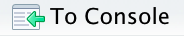(To Console) button to copy the command to the Console, where you can then edit it and run it.

Cleaning up

Sometimes the Console gets visually cluttered. You can easily solve that using the (broom) button. The History tab also has a broom button, if you want to clear your command history.

Autocomplete

As we start to write more code later, you’ll start to appreciate RStudio’s autocomplete feature. As you’re typing code, if you press Tab, RStudio will offer you all of the functions, variable names, etc. that match what you’ve typed so far. You can then either use the mouse or the keyboard arrows to scroll through the choices and choose the one you want.

Running code from within the file editor

We’ve learned about running R code from the RStudio Console, but usually your objective is to write R code that you can

Tip: Running segments of your code

RStudio offers you great flexibility in running code from within the editor window. There are buttons, menu choices, and keyboard shortcuts. To run the current line, you can

1. click on the Run button above the editor panel, or
2. select “Run Lines” from the “Code” menu, or
3. hit Ctrl+Return in Windows or Linux or ⌘+Return on OS X. (This shortcut can also be seen by hovering the mouse over the button). To run a block of code, select it and then Run. If you have modified a line of code within a block of code you have just run, there is no need to reselect the section and Run, you can use the next button along, Re-run the previous region. This will run the previous code block including the modifications you have made.

Errors and Warnings

Using R as a calculator

The simplest thing you could do with R is do arithmetic:

1 + 100

[1] 101

And R will print out the answer, with a preceding “[1]”. Don’t worry about this for now, we’ll explain that later. For now think of it as indicating output.

Like bash, if you type in an incomplete command, R will wait for you to complete it:

> 1 +

+

Any time you hit return and the R session shows a “+” instead of a “>”, it means it’s waiting for you to complete the command.

When using R as a calculator, the order of operations is the same as you would have learned back in school.

From highest to lowest precedence:

• Parentheses: (, )
• Exponents: ^ or **
• Divide: /
• Multiply: *
• Add: +
• Subtract: -

3 + 5 * 2

[1] 13

Use parentheses to group operations in order to force the order of evaluation if it differs from the default, or to make clear what you intend.

(3 + 5) * 2

[1] 16

This can get unwieldy when not needed, but clarifies your intentions. Remember that others may later read your code.

(3 + (5 * (2 ^ 2))) # hard to read
3 + 5 * 2 ^ 2       # clear, if you remember the rules
3 + 5 * (2 ^ 2)     # if you forget some rules, this might help

The text after each line of code is called a “comment”. Anything that follows after the hash (or octothorpe) symbol # is ignored by R when it executes code.

Really small or large numbers get a scientific notation:

2/10000

[1] 2e-04

Which is shorthand for “multiplied by 10^XX”. So 2e-4 is shorthand for 2 * 10^(-4).

You can write numbers in scientific notation too:

5e3  # Note the lack of minus here

[1] 5000

Mathematical functions

R has many built in mathematical functions. To call a function, we simply type its name, followed by open and closing parentheses. Anything we type inside the parentheses is called the function’s arguments:

sin(1)  # trigonometry functions

[1] 0.841471

log(1)  # natural logarithm

[1] 0

log10(10) # base-10 logarithm

[1] 1

exp(0.5) # e^(1/2)

[1] 1.648721

Don’t worry about trying to remember every function in R. You can simply look them up on Google, or if you can remember the start of the function’s name, use the tab completion in RStudio.

This is one advantage that RStudio has over R on its own, it has auto-completion abilities that allow you to more easily look up functions, their arguments, and the values that they take.

Typing a ? before the name of a command will open the help page for that command. As well as providing a detailed description of the command and how it works, scrolling to the bottom of the help page will usually show a collection of code examples which illustrate command usage. We’ll go through an example later.

Comparing things

We can also do comparison in R:

1 == 1  # equality (note two equals signs, read as "is equal to")

[1] TRUE

1 != 2  # inequality (read as "is not equal to")

[1] TRUE

1 < 2  # less than

[1] TRUE

1 <= 1  # less than or equal to

[1] TRUE

1 > 0  # greater than

[1] TRUE

1 >= -9 # greater than or equal to

[1] TRUE

Tip: Comparing Numbers

A word of warning about comparing numbers: you should never use == to compare two numbers unless they are integers (a data type which can specifically represent only whole numbers).

Computers may only represent decimal numbers with a certain degree of precision, so two numbers which look the same when printed out by R, may actually have different underlying representations and therefore be different by a small margin of error (called Machine numeric tolerance).

Instead you should use the all.equal function.

Further reading: http://floating-point-gui.de/

Variables and assignment

We can store values in variables using the assignment operator <-, like this:

x <- 1/40

Notice that assignment does not print a value. Instead, we stored it for later in something called a variable. x now contains the value 0.025:

x

[1] 0.025

More precisely, the stored value is a decimal approximation of this fraction called a floating point number.

Look for the Environment tab in one of the panes of RStudio, and you will see that x and its value have appeared. Our variable x can be used in place of a number in any calculation that expects a number:

log(x)

[1] -3.688879

Notice also that variables can be reassigned:

x <- 100

x used to contain the value 0.025 and and now it has the value 100.

Assignment values can contain the variable being assigned to:

x <- x + 1 #notice how RStudio updates its description of x on the top right tab
y <- x * 2

The right hand side of the assignment can be any valid R expression. The right hand side is fully evaluated before the assignment occurs.

Variable names can contain letters, numbers, underscores and periods. They cannot start with a number nor contain spaces at all. Different people use different conventions for long variable names, these include

• periods.between.words
• underscores_between_words
• camelCaseToSeparateWords

What you use is up to you, but be consistent.

It is also possible to use the = operator for assignment:

x = 1/40

But this is much less common among R users. The most important thing is to be consistent with the operator you use. There are occasionally places where it is less confusing to use <- than =, and it is the most common symbol used in the community. So the recommendation is to use <-.

Challenge 1

Which of the following are valid R variable names?

min_height
max.height
_age
.mass
MaxLength
min-length
2widths
celsius2kelvin

Solution to challenge 1

The following can be used as R variables:

min_height
max.height
MaxLength
celsius2kelvin

The following creates a hidden variable:

.mass

The following will not be able to be used to create a variable

_age
min-length
2widths

Challenge 2

Are R variable names case-sensitive?

Solution to challenge 2

Yes. You might have tested this by trying something like:

myvariable <- 5

MyVariable

Error in eval(expr, envir, enclos): object 'MyVariable' not found

Vectorization

One final thing to be aware of is that R is vectorized, meaning that variables and functions can have vectors as values. In contrast to physics and mathematics, a vector in R describes a set of values in a certain order of the same data type. For example

1:5

[1] 1 2 3 4 5

2^(1:5)

[1]  2  4  8 16 32

x <- 1:5
2^x

[1]  2  4  8 16 32

This is incredibly powerful; we will discuss this further in an upcoming lesson.

Managing your environment

There are a few useful commands you can use to interact with the R session.

ls will list all of the variables and functions stored in the global environment (your working R session):

ls()

[1] "args"          "dest_md"       "missing_pkgs"  "myvariable"   
[5] "required_pkgs" "src_rmd"       "x"             "y"            

Tip: hidden objects

Like in the shell, ls will hide any variables or functions starting with a “.” by default. To list all objects, type ls(all.names=TRUE) instead

Note here that we didn’t give any arguments to ls, but we still needed to give the parentheses to tell R to call the function.

If we type ls by itself, R will print out the source code for that function!

ls

function (name, pos = -1L, envir = as.environment(pos), all.names = FALSE, 
    pattern, sorted = TRUE) 
{
    if (!missing(name)) {
        pos <- tryCatch(name, error = function(e) e)
        if (inherits(pos, "error")) {
            name <- substitute(name)
            if (!is.character(name)) 
                name <- deparse(name)
            warning(gettextf("%s converted to character string", 
                sQuote(name)), domain = NA)
            pos <- name
        }
    }
    all.names <- .Internal(ls(envir, all.names, sorted))
    if (!missing(pattern)) {
        if ((ll <- length(grep("[", pattern, fixed = TRUE))) && 
            ll != length(grep("]", pattern, fixed = TRUE))) {
            if (pattern == "[") {
                pattern <- "\\["
                warning("replaced regular expression pattern '[' by  '\\\\['")
            }
            else if (length(grep("[^\\\\]\\[<-", pattern))) {
                pattern <- sub("\\[<-", "\\\\\\[<-", pattern)
                warning("replaced '[<-' by '\\\\[<-' in regular expression pattern")
            }
        }
        grep(pattern, all.names, value = TRUE)
    }
    else all.names
}
<bytecode: 0x7fd1d26258e0>
<environment: namespace:base>

You can use rm to delete objects you no longer need:

rm(x)

If you have lots of things in your environment and want to delete all of them, you can pass the results of ls to the rm function:

rm(list = ls())

In this case we’ve combined the two. Like the order of operations, anything inside the innermost parentheses is evaluated first, and so on.

In this case we’ve specified that the results of ls should be used for the list argument in rm. When assigning values to arguments by name, you must use the = operator!!

If instead we use <-, there will be unintended side effects, or you may get an error message:

rm(list <- ls())

Error in rm(list <- ls()): ... must contain names or character strings

Tip: Warnings vs. Errors

Pay attention when R does something unexpected! Errors, like above, are thrown when R cannot proceed with a calculation. Warnings on the other hand usually mean that the function has run, but it probably hasn’t worked as expected.

In both cases, the message that R prints out usually give you clues how to fix a problem.

R Packages

It is possible to add functions to R by writing a package, or by obtaining a package written by someone else. As of this writing, there are over 10,000 packages available on CRAN (the comprehensive R archive network). R and RStudio have functionality for managing packages:

• You can see what packages are installed by typing installed.packages()
• You can install packages by typing install.packages("packagename"), where packagename is the package name, in quotes.
• You can update installed packages by typing update.packages()
• You can remove a package with remove.packages("packagename")
• You can make a package available for use with library(packagename)

Challenge 3

What will be the value of each variable after each statement in the following program?

mass <- 47.5
age <- 122
mass <- mass * 2.3
age <- age - 20

Solution to challenge 3

mass <- 47.5

This will give a value of 47.5 for the variable mass

age <- 122

This will give a value of 122 for the variable age

mass <- mass * 2.3

This will multiply the existing value of 47.5 by 2.3 to give a new value of 109.25 to the variable mass.

age <- age - 20

This will subtract 20 from the existing value of 122 to give a new value of 102 to the variable age.

Challenge 4

Run the code from the previous challenge, and write a command to compare mass to age. Is mass larger than age?

Solution to challenge 4

One way of answering this question in R is to use the > to set up the following:

mass > age

[1] TRUE

This should yield a boolean value of TRUE since 109.25 is greater than 102.

Challenge 5

Clean up your working environment by deleting the mass and age variables.

Solution to challenge 5

We can use the rm command to accomplish this task

rm(age, mass)

Challenge 6

Install the following packages: ggplot2, plyr, gapminder

Solution to challenge 6

We can use the install.packages() command to install the required packages.

install.packages("ggplot2")
install.packages("plyr")
install.packages("gapminder")

Key Points

• Use RStudio to write and run R programs.

• R has the usual arithmetic operators and mathematical functions.

• Use <- to assign values to variables.

• Use ls() to list the variables in a program.

• Use rm() to delete objects in a program.

• Use install.packages() to install packages (libraries).